Bayesian Optimisation

Optimise a function with probabilities.

---

Finding the extrema of a function, maxima or minima, is a thing that it’s often very useful to do. For instance we want some input, $x^\ast$, to $f$ such that

\[x^\ast = \rm{argmax}\:\:f(x)\]

In machine learning in particular we find ourselves doing this a lot, for instance we have some set of model parameters we want to learn from data by finding the values which minimise a loss function. The most common way of doing this is by gradient descent¹. This is an extremely powerful method, especially since for lots of ML applications the loss function will have some nice properties like smoothness, and in some cases convexity.

Unfortunately gradient descent, as the name implies, requires that we have knowledge about the derivative of the function, and there are lots of cases where we don’t have this information. To look again at machine learning, we will often have a second type of parameter in our model, the hyper-parameters, which specify the model configuration and which we can’t optimise by gradient descent. These hyper-parameters might be things like the number of trees in a random forest or the regularisation strength of a linear model, which don’t have gradients we can easily compute with respect to the loss function and are very expensive to evaluate. This is a problem. And it says a lot about this problem that one common way it’s solved in practice is by just trying random values of the hyper-parameters until you hit a good one. All’s not lost however, Bayesian Optimisation to the rescue.

The idea behind Bayesian Optimisation is to try to find the maximum of some black-box function by getting values from that black-box and using those to inform where we should look next to maximise our probability of finding $x^\ast$. We do this by using some prior over the kind of functions that our black-box function comes from, and as we observe more points we update this belief. As we get more data we better constrain the functions that could potentially be in the box, and so we get a better idea of where $x^\ast$ might be.

Let’s look at a concrete example. Say that we’ve got this function that I just made up,

\[f(x) = 5 \sin(3x) + 0.3x^2 - 2x\]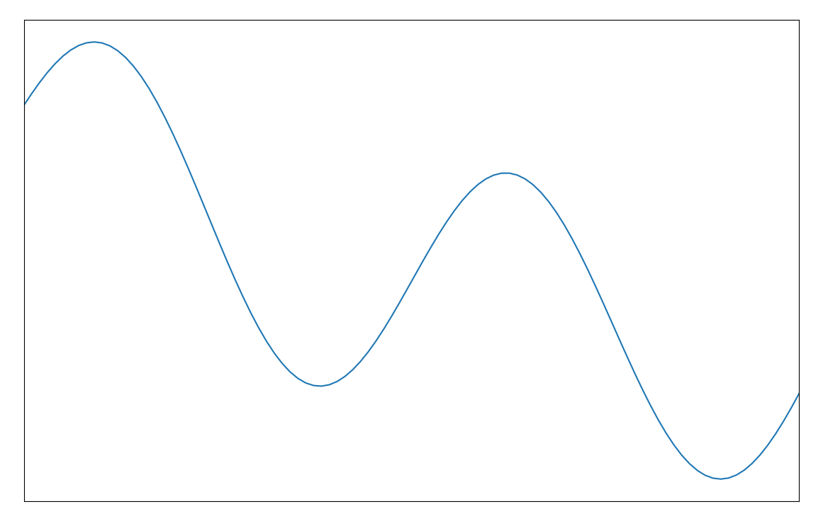

and we’re looking for $x^\ast$ over a particular domain, given that all we can do is make noisy observations of $f(x)$.

We’ll begin, before observing any data, by making some assumptions about the class of functions from which $f(x)$ has itself been drawn. Specifically we place a Gaussian Process prior on this function.² For those unfamiliar with GPs, they’re a very flexible class of model which allow us to assign probabilities to functions given observations. They also allow us compute the mean and the standard deviation of the values of these functions for a particular input, for instance:

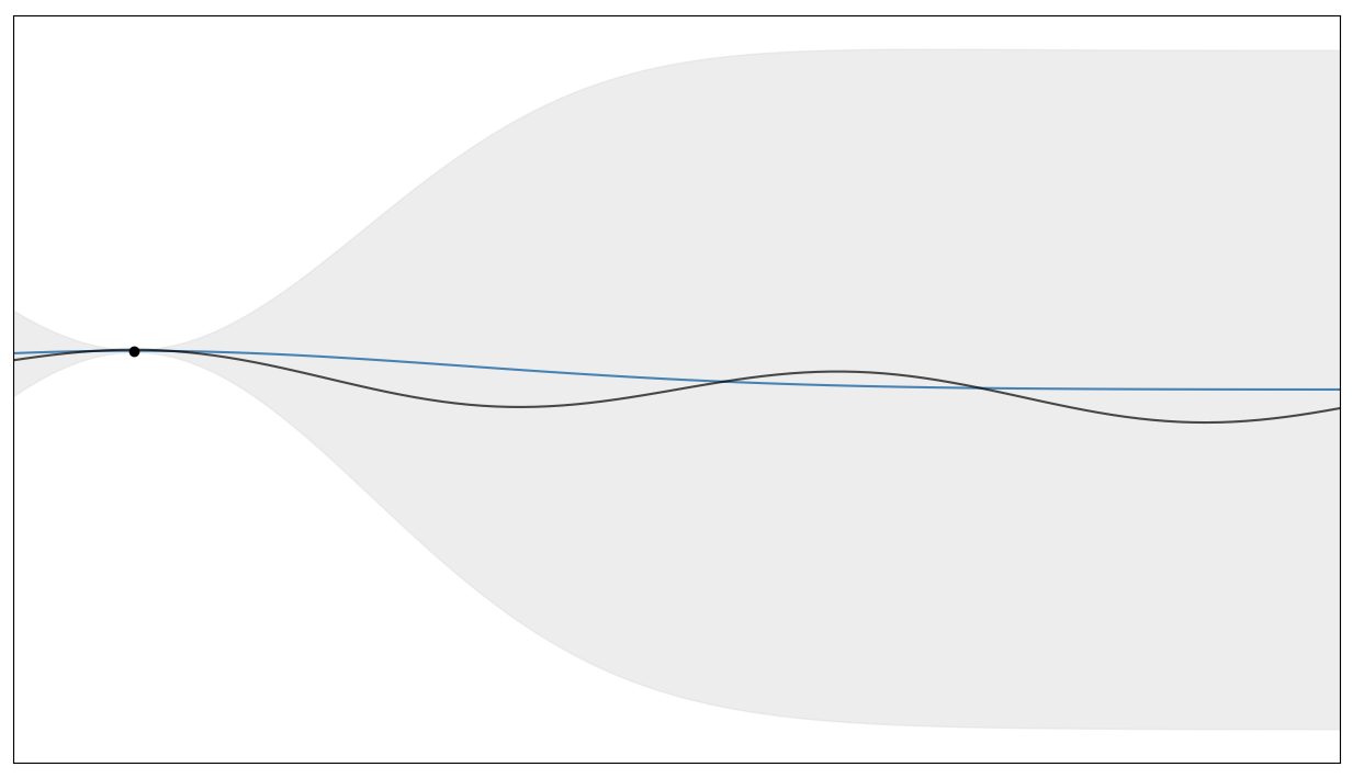
Here we’ve observed the black point from the function indicated by the black line, and given this observation the GP estimates the mean of the hidden function to be the blue line, with the shaded region indicating the standard deviation of its prediction.

Using this information we build what’s called an acquisition function, a function which tells us where to next look for the maximum given the values we’ve already observed. There are a lot of choices for the acquisition function, but a common choice is the Expected Improvement. EI is defined

\[\rm{EI}(x) = \mathbb{E}[(f(x) - x^\ast)^+]\]

where $f(x)^+ = \max(f(x), 0)$. So the EI tells us how much greater than the currently observed maximum we should expect the function to be at a given point. And, conveniently, we can evaluate this quantity in closed form³

\[\rm{EI}(x) = \Delta(x)^+ + \sigma(x)\phi\bigg(\frac{\Delta(x)}{\sigma(x)}\bigg) - |\Delta(x)|\psi\bigg(\frac{\Delta(x)}{\sigma(x)}\bigg)\]

where $\Delta(x) = f(x) - x^\ast$, $\phi$ is the PDF of a standard normal distribution, and $\psi$ is its CDF.

Using the GP and the EI, we can write and algorithm to find the maximum,

1. Compute a GP prior on the hidden function.
2. Use this to compute the EI.
3. Sample a new point at the maximum of the EI.
4. Recompute the GP in light of the new data.

And continue this process for a set number of steps. The gif below shows this process for 10 iterations over the function I showed above,

The top panel show the function, along with the data, the GP, and a dotted line showing the location of the true $x^\ast$. The lower panel shows the acquisition function at each step, its maximum being the location where we should next sample. As you can see the whole process is pretty efficient, converging to $x^\ast$ in fewer than 15 steps.

The code for all of this is here. If, sensibly, you’d like to use a GP implementation that I haven’t written you have a few choices, MOE for example.

---