Gradient Descent

$\nabla$

There’s a strong argument to be made that gradient descent is the most useful algorithm ever invented. The idea behind it is simple and powerful. It is premised on the (perhaps counter-intuitive) fact that it is possible to perform a global optimisation of a function based solely on local information.¹

Given some function $f: \mathbb{R} \rightarrow \mathbb{R}$, let’s say we want to find the input value, $x$, such that the output, $y$, is minimised; a pretty common thing to want to do. The way we do this is by starting off at some point, evaluating the derivative of the function ($\nabla f$) at that point, and moving in the direction of steepest descent as indicated by that derivative. We keep doing this until the derivative is (close to) 0. The derivative is our piece of local information, but by following this recipe we can find the minimum of the function.²

To put this in more mathematical terms, we can define the steps we take at each iteration,

where $\alpha$ is a learning rate, a value that we can tune that determines how large our changes to $x$ will be. For a small enough learning rate we always improve our current position. So we have an example let’s take this function here,

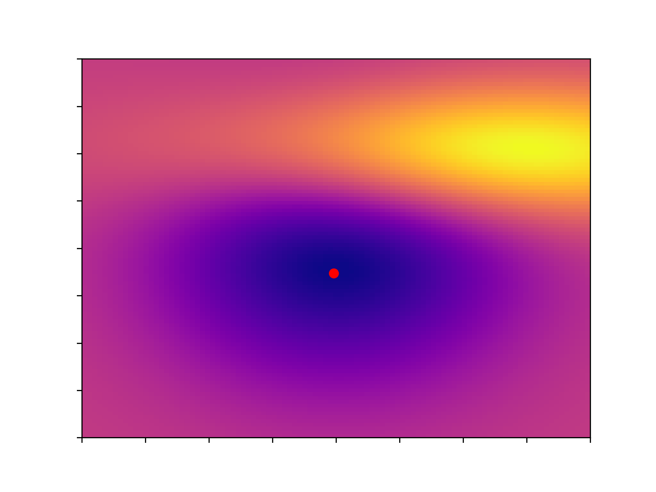
Here’s a nice smooth function (for the sake of transparency it’s 2 normals glued together), with a single global minimum, indicated with a red dot. We can write a gradient descent function in Python very simply, and try it out,

def descent(f, x, alpha=0.001, maxiter=1000):
  i = 0
  xk = None
  f_grad = grad(f)
  while i < maxiter and xk != x:
    xk = x
    x = x - alpha * f_grad(x)
    i += 1
  return x

Here we’ve got a very simple implementation of gradient descent, which makes use of the (almost magical) Python autograd library. This library gives us the function, grad, which takes in a Python function and returns a function that will tell us its gradient. This makes life very convenient. Using that function above we get something like this,

We start off on the side of that hill, and by following the gradient we eventually get down to the minimum. One thing you’ll notice is that, as the slope becomes shallower our point moves more slowly, its steps become more tentative. We start off with big, bold steps towards the minimum but soon find that our progress slows. How do we get past this?

It turns out that you can make a big improvement³ at very little expense by using momentum, in effect giving our gradient a little bit of short-term memory. Using this method our updates become,

In the case that $\gamma=0$ we recover our previous algorithm, however if we set $\gamma=0.99$ then we remember the direction of our previous steps, and we see that our method seems greatly improved. Coding it up requires only a small change

def momentum(f, x, alpha=0.001, gamma=0.99, maxiter=1000):
  i = 0
  v = 0
  xk = None
  f_grad = grad(f)
  while i < maxiter and xk != x:
    xk = x
    v = gamma * v + alpha * f_grad(x)
    x = x - v
    i += 1
  return x

but the increase we see is striking,

As promised we converge more quickly, in fact it only takes one third as many steps.

There are two common analogies used to describe these 2 algorithms: traditional gradient descent is a person lost in fog on a hill-side, they can’t see where they’re going, so they look at the direction of the slope under their feet and take a small step downhill. Momentum is more like a ball rolling down the hill, its inertia helping to smooth out its descent and to keep it moving quickly. I think you can see the validity of these analogies in the GIFs above.

What if we take these out of the realm of analogy and try it out for real? NASA provides raster data of the elevation of most of the Earth. So we can pull down this topographic data and try to do gradient descent on it directly. Annoyingly Ireland doesn’t quite fit on one raster tile, it’s a bit cropped at the edges, but in the end this is the data that we get

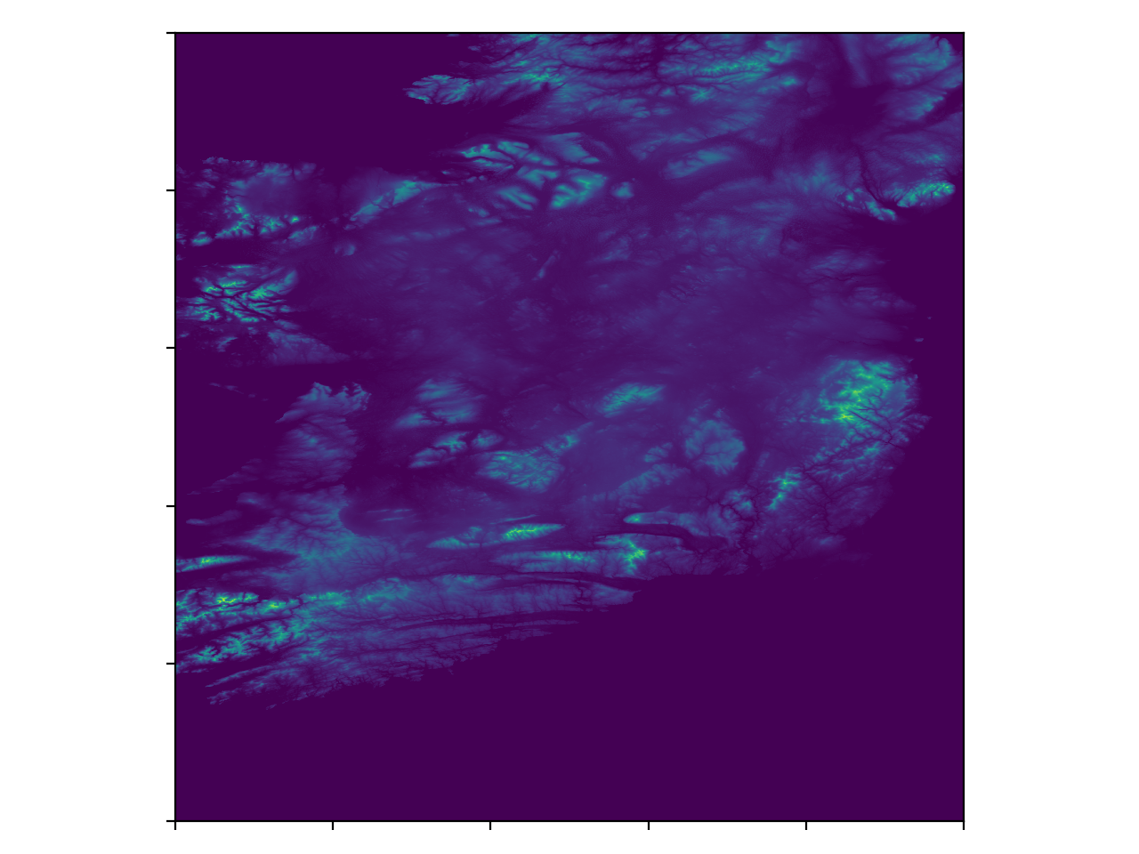
Spooky. To do gradient descent on this we’ll need to compute the gradients, since we can’t do autograd on Ireland,

def grad(pt, eps=1e-3):
    x, y = pt[0], pt[1]
    x_p = (elevation((x + eps, y)) - elevation((x, y))) / eps
    y_p = (elevation((x, y + eps)) - elevation((x, y))) / eps
    return x_p, y_p

where the elevation function just returns the value from our topographic raster array.

Now we have all we need to use the two functions above. Let’s start off with the simple gradient descent, our hill-walker lost in the fog. I’ve chosen to start him off at the top of Mt. Leinster, a fairly big mountain near my home, and let him wander from there. You can see the results here,⁴

As you can see things start out reasonably well, it starts off following the steep slope at the top of the mountain, and soon joins up with a river (the wonderfully named River Mountain) which is a sign that we’ve found a good route. Things go awry once we hit the bottom of the mountain; once we get into the valley and the slope becomes shallower there’s not enough gradient information to point the hill-walker in the right direction, so it stalls.

Let’s try the same thing with momentum.

Using momentum we see that the motion is a lot smoother, the ball rolls down hill and eventually into the River Barrow.⁵

The recent increasing interest in neural networks has led to a lot of focus on gradient descent methods, and they all spring from momentum in some sense. Conjugate gradient, ADAM, AdaGrad, and many others are just a small extension of the idea which inspired momentum⁶, and I imagine I’ll revisit them in another post at some point.