Introduction to Gaussian Processes, 1

Gaussian Processes (GPs) are a really flexible, really powerful class of models that have seen a lot of use in the last fifteen or twenty years. In this post I’d like to go through the background to these models, what they are, and how they work; primarily so I can try straighten out some of these ideas in my own head.

This is the first of what I reckon will be three posts, and here I’ll really just go through some simple ideas in model fitting, gearing up for a discussion of GPs.

Regression

In regression problems our aim is to try to predict some target variable, $y$, given some input, $x$. Let’s assume that there is some hidden function which we want to model, and let’s begin with the univariate case, $f: \mathbb{R} \rightarrow \mathbb{R}$. We have some training data, $\mathbf{x} = [x_1,\dots,x_n]^T$ and $\mathbf{y} = [y_1,\dots,y_n]^T$ where $y_i = f(x_i)$, and we want to make predictions of $y$ at some new, unobserved points $x_\ast$.

The best place to start is at the beginning with everyone’s favourite, a linear model

If we assume that the hidden function generating our data is linear, then the easiest case is if we have two data points. Given two observations we can solve the resultant pair of simultaneous equations, and get this

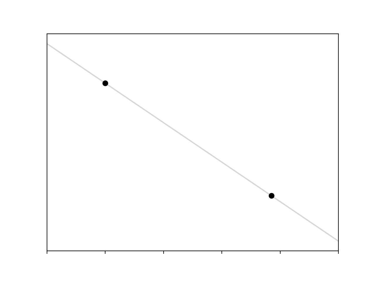
Cool.

Things get a lot worse if we add another point that doesn’t sit on the line defined by the other two. Now we have an overdetermined system of equations, 3 equations with 2 unknowns, so there are 3 lines we can fit

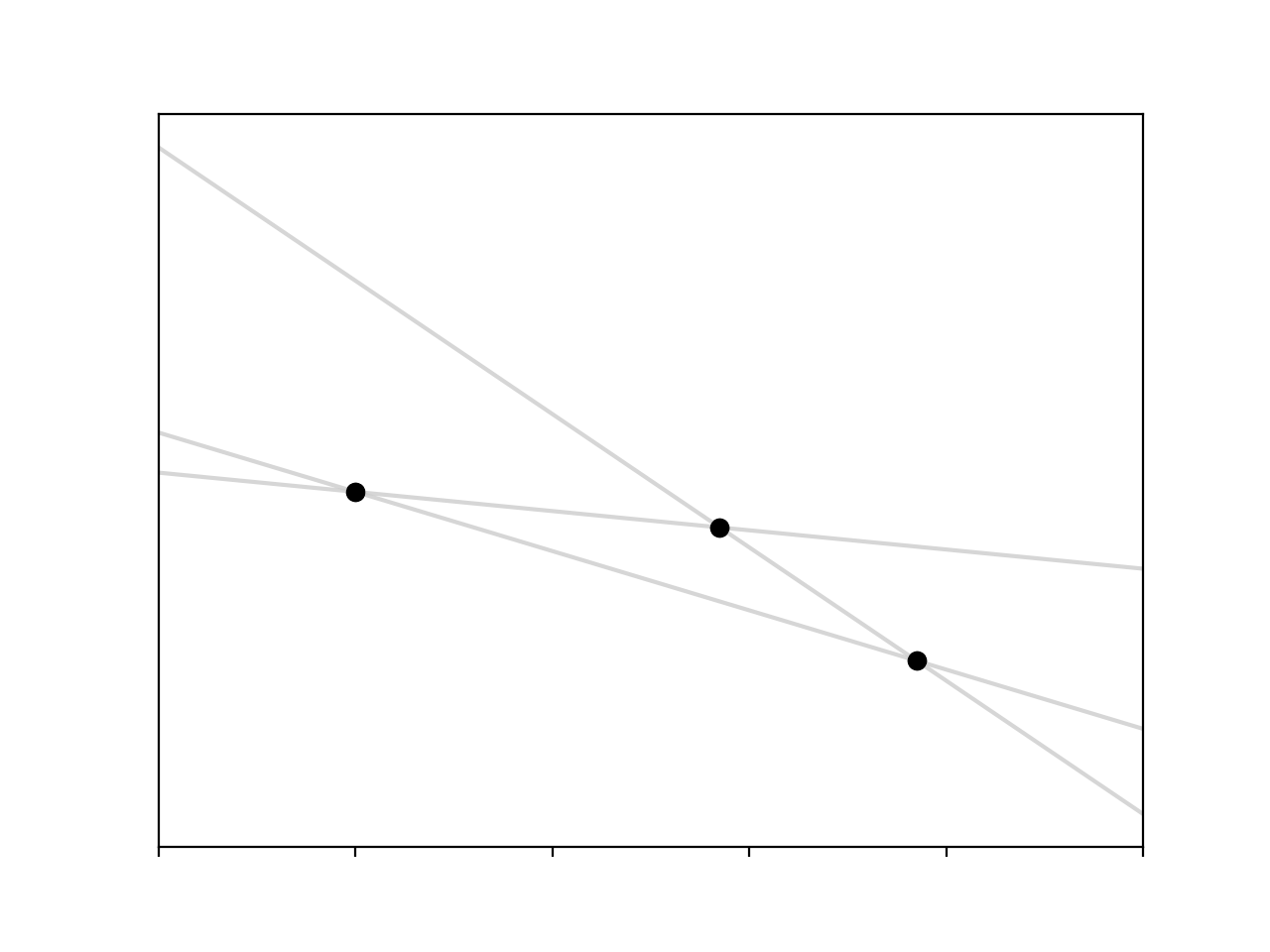
Which line is the ‘correct’ one? This was a real problem for people like Gauss, Laplace, and Legendre, the first scientists concerned with trying to fit models to observation.¹ Sticking with the assumption that our data truly comes from a linear function then the reason that our points don’t sit on the same line is that there are some un-modeled sources of variance in our observational set-up. To account for this we add another term to our model which explains the discrepancy,

Now we have $N+2$ parameters, we have an $\epsilon$ for each data point along with $m$ and $c$. We get around this by making another assumption, that $\epsilon$ is a random variable drawn from some probability distribution. Often we assume that $\epsilon$ is drawn from a normal distribution with some mean and standard deviation,²

Now we can solve the equations (by some method) and find the line of best fit to these points.³

I think it’s actually more instructive to look at things from the other perspective, what if we only had one observation? In that case we’re left with an underdetermined system, we now have one equation in two unknowns, $m$ and $c$.

All is not lost though, we can still fit a linear model, provided we are willing to make some assumptions about our parameters. For instance, let’s assume that the intercept is distributed according to a normal distribution. This is very similar to what we did in the overdetermined case, we substitute some variable with a probability distribution, though the variables have very different interpretations – in the overdetermined case the variable we introduce is a kind of noise model, in this case it’s one of our parameters. Based on this assumption we can sample intercepts from the probability distribution and fit possible lines to our point

px, py = np.random.rand(2)
x = np.linspace(0, 1, 100)

for i in range(100):
        c = np.random.randn()
        m = (py - c) / px
        y = m * x + c
        plt.plot(x, y, c='0.8', alpha=0.7)

plt.plot(px, py, 'ok')

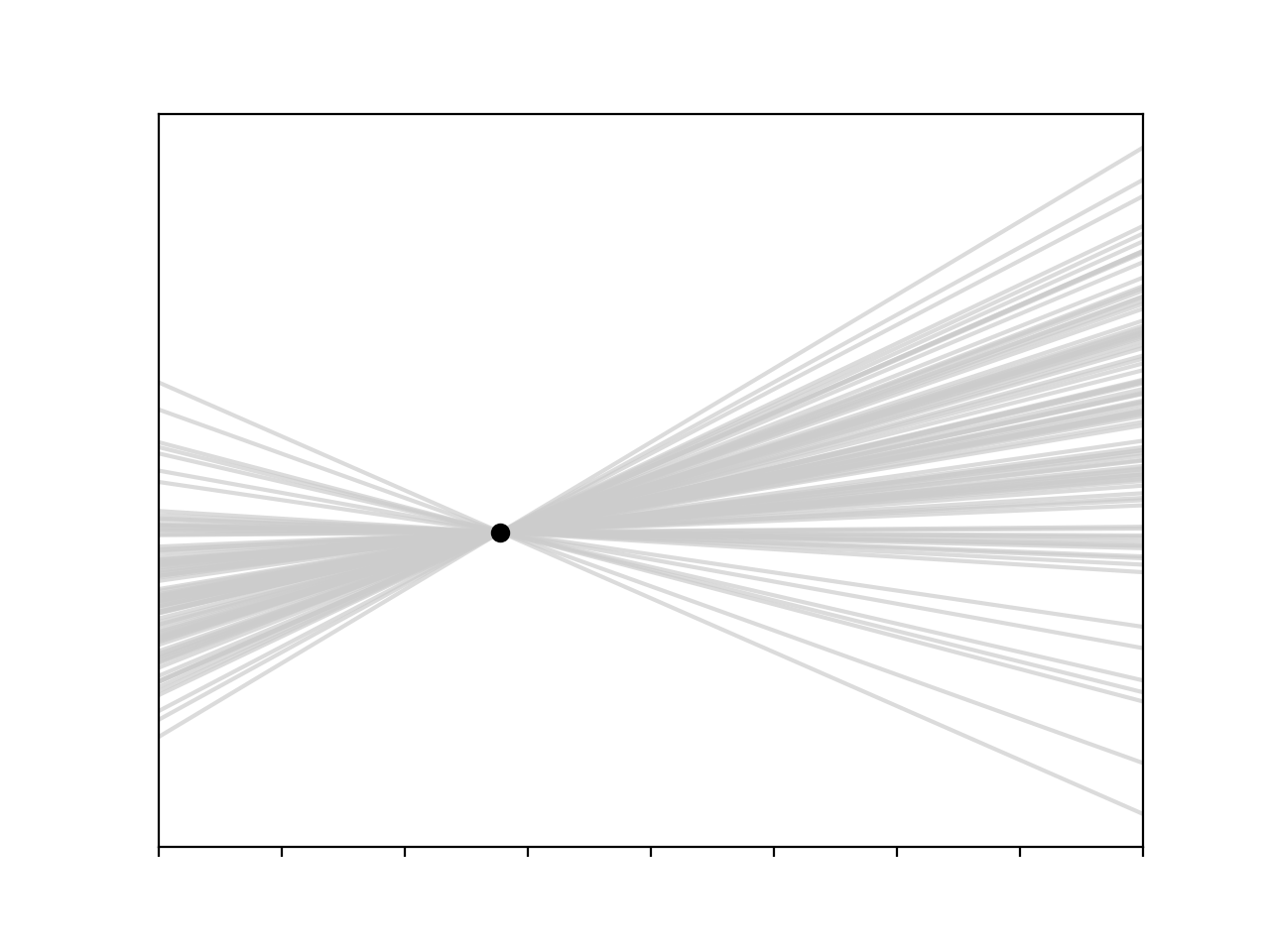
I’m a big fan of this model. It’s fairly transparent, and it agrees well with our intuitions – if we make some assumption about one of our parameters and combine that assumption with our data we can generate some confidence about where our true function lies, we can be really confident near the observation and less so further away. It’s nice to see that in a plot.

Now that we’re putting probability distributions over the parameters of our model we’re straying into Bayesian territory, we can begin to look at linear models for which we have some prior belief about the parameters; let’s stick with Gaussian priors. Once we’ve observed some data we can update our belief using Bayes rule, and the nice thing here is that since we have begun with a Gaussian prior and our likelihood is Gaussian, and the product of Gaussians is Gaussian,⁴ then our posterior will be Gaussian and we can analytically solve for its mean and covariance. This is exceptionally convenient.

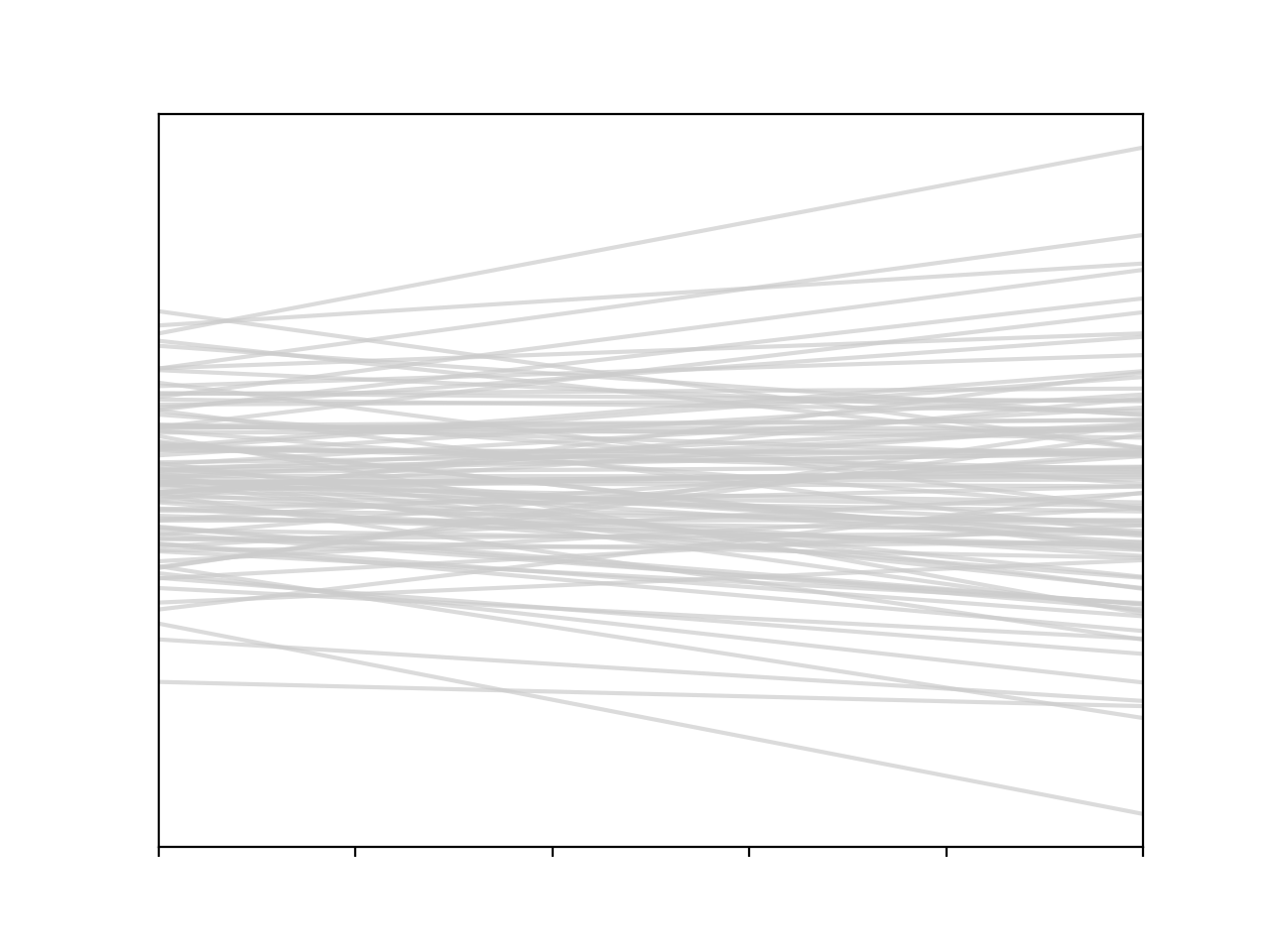
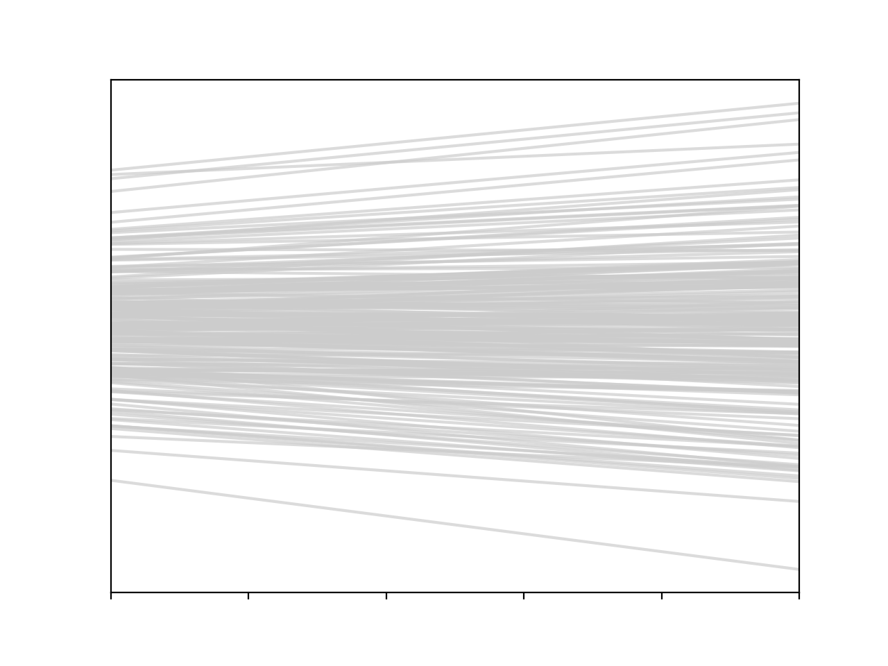
We can also draw from the priors, combine this with our predictive model, and sample some $f$’s that are consistent with our beliefs

for i in range(100):
        c, m = np.random.normal(size=2)
        y = m * x + c
        plt.plot(x, y, c='0.8', alpha=0.7)

So what we’ve got here, in a more succinct notation is

where $\mathbf{w}$ is a stochastic variable, a matrix containing our weights $[c, m]$, and $\phi$ is our basis function⁵, which in this simple case is

Looking at things from this perspective something interesting happens. We can see that $\phi(\mathbf{x})$ is a deterministic matrix, solely reliant on the data (given a choice of basis), and $\mathbf{w}$ is a random variable comprised of two Gaussians. The cool thing is that we can use the standard (and unique) properties of Gaussians to combine all of this and write down the probability distribution that is implied over $f$. For example if we know that $\mathbf{w}$ is sampled from a Gaussian, $\mathcal{N}(0, \, \alpha\mathbf{I})$, then we can say that $f$ is sampled from a multivariate Gaussian

In other words, rather than sampling from our priors and putting these values into our prediction function, we can sample functions directly from this multivariate Gaussian, and get the same thing⁶

def phi(x): return np.vstack((x**0, x**1))

k = phi(x).T.dot(phi(x))
for i in range(100):
        f = np.random.multivariate_normal(np.zeros(x.size), k)
        plt.plot(x, f, c='0.8', alpha=0.7)

This is the real core of the shift in thinking around GPs. We have moved from putting probability distributions over parameters and drawing samples, to putting probability distributions over the functions themselves. It’s a bit of a mind-blowing thing to do.

I’m sure that this isn’t all perfectly clear at the moment, I’m not sure I’ve done a particularly good job explaining what’s going on here. Hopefully things will become clearer in part 2, where I’ll move on to the real nuts and bolts of GPs.