Introduction to Gaussian Processes, 2

In this post I want to take a deeper look at what a Gaussian Process is doing under hood.

At the end of the last post we had gotten to the idea that, rather than treating the parameters of a model as probability distributions, we could write down a probability distribution over functions, and sample directly from that. Concretely, we left things with the observation that, given a basis function, $\phi(\mathbf{x})$, we could write down the probability distribution over functions in this basis¹ as,

Sampling from this multivariate Gaussian will give us functions that are drawn from the span of the basis $\phi$.

To clarify what I mean by this let’s look at the case of a 2D Gaussian,

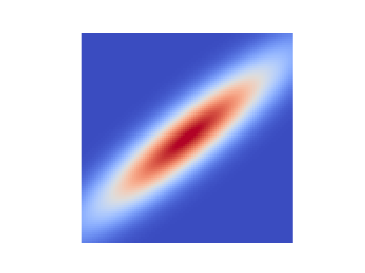
This Gaussian has zero mean², and some covariance which we’ll call $\mathbf{K}$, $\mathcal{N}(\mathbf{0},\, \mathbf{K})$. For a 2D Gaussian $\mathbf{K}$ is a $2\times2$ matrix, and it’s clear that this $\mathbf{K}$ has some non-trivial structure, which is to say there are non-zero elements off the main diagonal. We can take draws from this distribution, pairs of values, let’s call them $(x_1, \, x_2)$. One thing we can look at is how setting $x_1$ to a given value affects $x_2$.

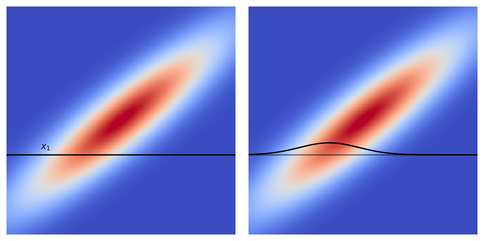
Looking at the diagram we see that setting $x_1$ to some value constrains $x_2$ to be drawn from (surprise surprise) a Gaussian distribution, with different Gaussians for different $x_1$’s.³ So by setting $x_1$ we can get an estimate for $x_2$, along with a variance. Let’s do that and plot up the results,

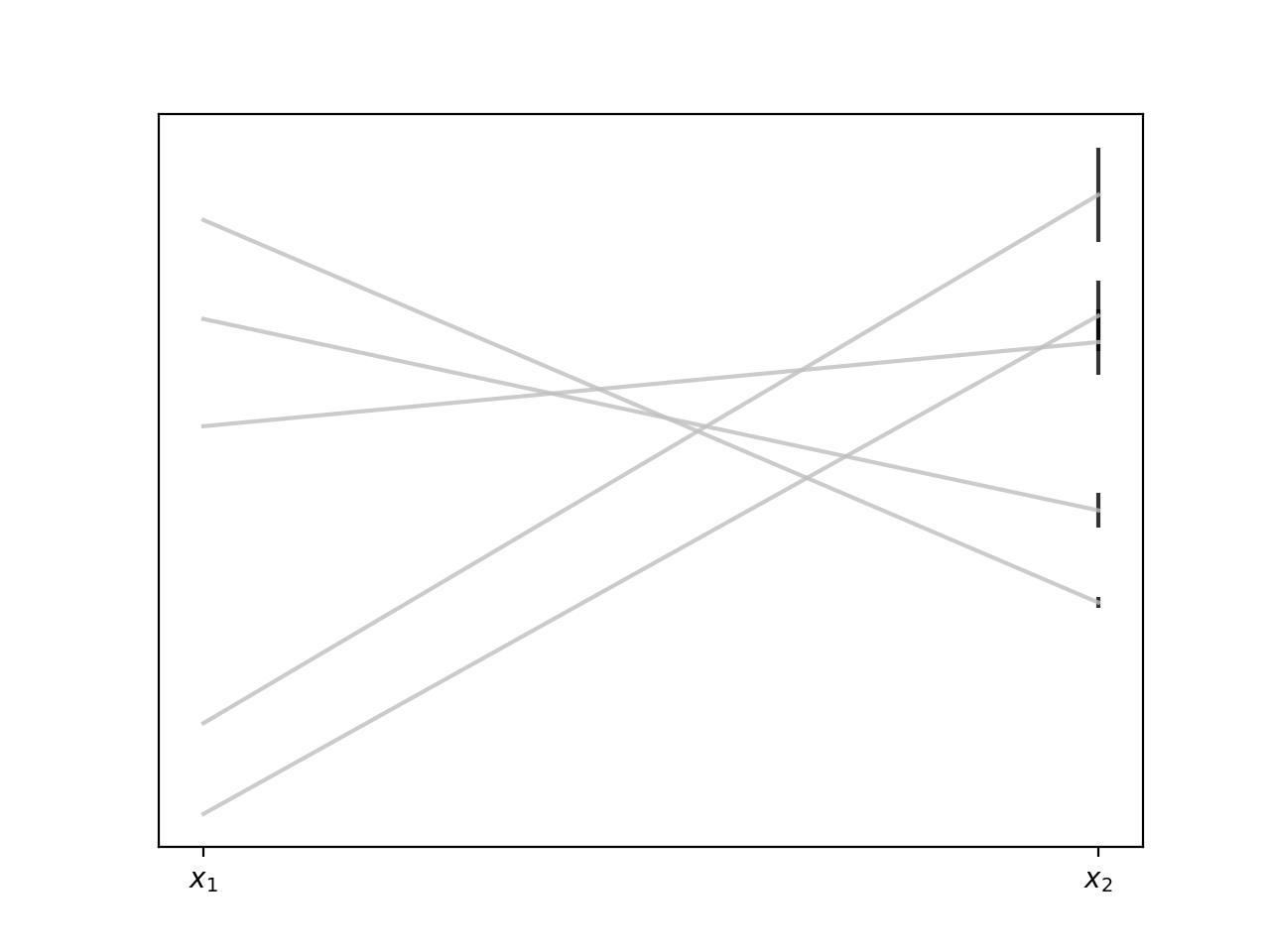
Viewed this way our samples are really samples from a distribution that generates pairs of 2D points. The important thing to bear in mind here is that the kind of points (lines) we get out (their slopes, intercepts, how varied they are) is entirely determined by the structure of the covariance matrix $\mathbf{K}$. We saw in the last post how we can build covariance matrices from basis functions, but there’s nothing that says we have to do things that way, we can build $\mathbf{K}$ by any method we like,⁴ and it will determine the kinds of functions we draw from the distribution.

Let’s look at a bigger example, let’s go from a 2D Gaussian to a 100D Gaussian.⁵ Now we need to specify a $100 \times 100$ matrix for $\mathbf{K}$. To do this we use a kernel function (the covariance matrix is often called the kernel), and one of the most common kernel functions is the Squared Exponential Kernel

Here $x$ and $x’$ are the values between which we want to determine the covariance, $\sigma$ is a scaling factor, and $l$ is the length scale of our covariance. Setting $\sigma$ and $l$, we can use this kernel to compute the covariance between pairs of points and populate our kernel matrix. It will end up having a structure like this

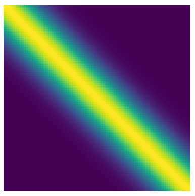
Here we see every point has covariance $1$ with itself (trivially), decreasing covariance with points nearby, and no covariance with distant points. Let’s take draws from a Gaussian with this covariance structure

def gaussian(C):
        '''
        return draw from a 0 mean gaussian with given covariance
        '''
        return np.random.multivariate_normal(np.zeros(len(C)), C)


def sq_exp_kernel(x, x_d, theta=[1, 1]):
        '''
        exponentiated quadratic kernel
        '''
        sig, l = theta
        x = x.reshape(-1,1)
        x_d = x_d.reshape(-1,1)

        sqdist = (np.sum(x**2, 1).reshape(-1, 1) +
                  np.sum(x_d**2, 1) -
                  2 * np.dot(x, x_d.T))

        return sig**2 * np.exp(-0.5 * (1 / l**2) * sqdist)


x = np.linspace(-1, 1, 100)
k = sq_exp_kernel(x, x)

for i in range(10):
    plt.plot(x, gaussian(k))

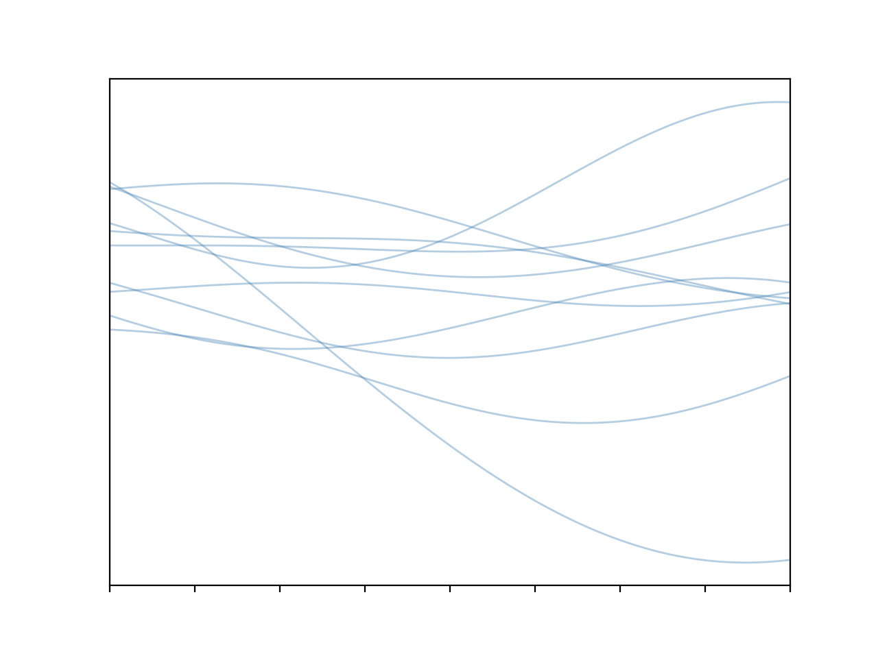
Cool! We get some nice, smoothly varying functions. The fact they vary in such a smooth way is a direct result of that covariance structure, points nearby will tend to vary together, hence no jagged lines. This is all well and good but what we’re missing here is the capacity to condition our distribution on data; once we’ve observed a data point in a given location that should constrain the types of functions that we consider valid in that region. And the way that we do this is by leveraging a very nice property of Gaussians, the fact that they are closed under conditioning.⁶

What we want to do is learn the probability distribution over functions given the training data. Concretely we would like to get the distribution of possible values at some test points, $x_\ast$, given the values at training points, $x$. The key idea of a Gaussian Process is that we model the underlying distribution of $x$ and $x_\ast$ as one big multivariate normal distribution. This joint distribution of test and training data will require a covariance matrix of dimension $|x| + |x_\ast|$. Using this distribution we construct the conditional probability $P(x_\ast|x)$, and because of the conditioning property we know this distribution will be Gaussian.

This joint probability density over training and test points is

This kernel matrix is how information is passed between the training data and the test points. From this we can get

That’s a bit of a mouthful, but by sampling from this distribution we can get functions which are conditioned on our observation⁷

x = np.random.random((1,1))
y = np.random.random((1,1))

x_s = np.linspace(-2, 2, 100)

kss = sq_exp_kernel(x_s, x_s)
ksx = sq_exp_kernel(x_s, x)
kxs = sq_exp_kernel(x, x_s)
kxx = sq_exp_kernel(x, x)
inv = np.linalg.inv

mu = ksx.dot(inv(kxx)).dot(y)
C = kss - ksx.dot(inv(kxx)).dot(kxs)

for i in range(10):
    plt.plot(x_s, np.random.multivariate_normal(mu, C))

plt.plot(x.ravel(), y.ravel(), 'ok')

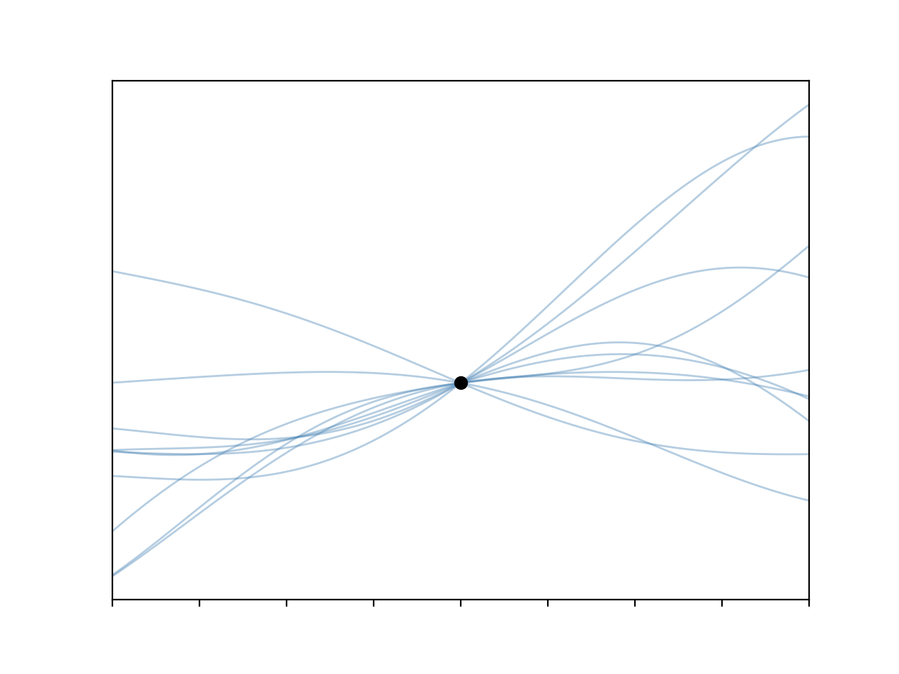
I have to admit I really like these plots.

So the last thing to cover is what to do with the two free parameters in the kernel function. These two control the amplitude of the functions, $\sigma$, and their length-scale (‘wiggliness’), $l$. Thankfully this isn’t too tricky, we can write down a likelihood function for our GP

and we can optimise by this gradient descent with respect to $\sigma$ and $l$. So let’s wrap things up by doing that for a toy problem. To start out we’ll draw some data from a hidden function

def f(x):
        return 2*np.sin(3*x) - np.cos(5*x) + x**2

def get_data(n_points):
        x = np.random.uniform(-2, 2, n_points)
        x.sort()
        u = 0.5
        y =  f(x) + np.random.randn(n_points) * u
        return x, y, u

Then code up that messy log likelihood there

def logl(theta, x, y, u, x_test):
        x = x.reshape(-1, 1)
        K = sq_exp_kernel(x, x, theta) + np.eye(len(x))*u**2
        y = y.reshape(-1, 1)
        L =    ( - 0.5 * np.dot(np.dot(y.T, np.linalg.inv(K)), y)
                 - 0.5 * np.log(np.linalg.det(K + 1e-6 * np.eye(len(x))))
                 - 0.5 * len(x) * np.log(2 * np.pi))[0][0]

        return L if np.isfinite(L) else 1e25

In general this is a terrible function, and you definitely don’t want to do things this way. Computing the determinent of $\mathbf{K}$ is a really bad call, the complexity goes as something bigger than $\mathcal{O}(n^{2.3})$, and the conditioning is terrible, even for this toy problem you’ll notice that I’m adding a small constant to the diagonal to try to keep things from breaking. Still, it’ll do for this example. Last thing is to stick this into an optimiser and solve for $\theta = (\sigma, l)$. Since most optimisers are minimisers, but we want the maximum likelihood, we’ll take the negative of this quantity and optimse that

nll = lambda *args: -1 * logl(*args)
result = opt.minimize(nll, [1, 1], args=(x, y, u, x_s))

Done. And presuming that didn’t fall over we should get something like this

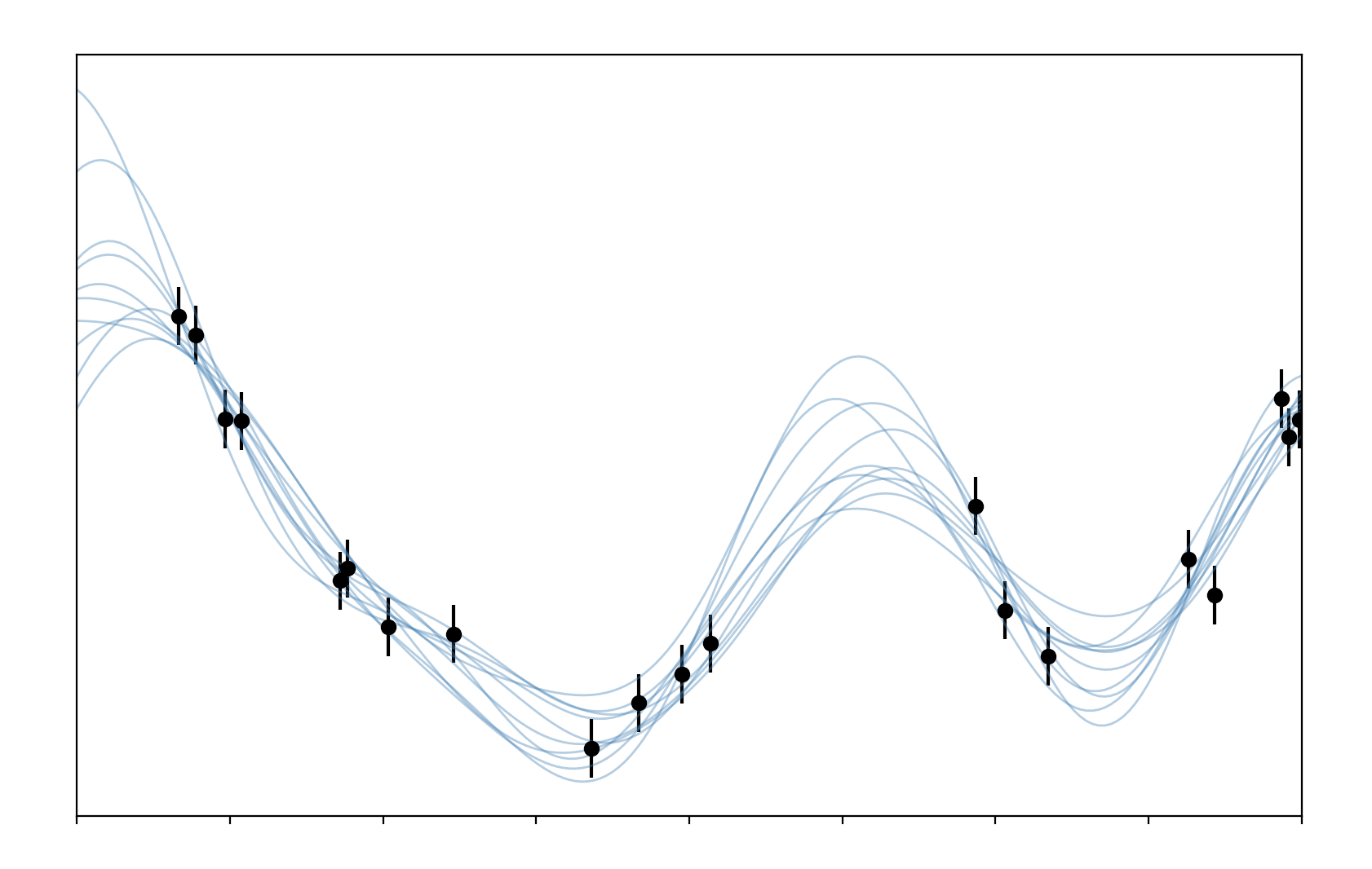
We can see that the draw from our GP match the data pretty well throughout, spreading out where we have no data to indicate our uncertainty about the possible values in this region. All of this code can be found here.

Now that we’ve rolled our own GP I feel I’ve got a clearer idea on what’s going on inside of them. In the next (and last) post I’ll cover using proper GP packages to fit models to real data.