Introduction to Gaussian Processes, 3

In this post I want to wrap up the short series on GPs by discussing the common GP packages in Python, and showing how to model some real data.

There are a lot of GP packages available in Python, you can find a pretty thorough comparison of a couple of the big ones in this paper. Briefly, and far from exhaustively, here are a couple of the GP tools

• scikit-learn: Scikit is the fist thing that comes to mind when you think of ML in Python, and conveniently it has a GP implementation. It doesn’t provide very many kernels out of the box, but you can add your own pretty easily.

• GPy/GFlow: GPy was developed by the group at Sheffield, and GPFlow is a reimplementation of GPy with a TensorFlow backend. It’s a pretty state-of-the-art tool box for all things GP, with a huge number of algorithms for applying GPs.

• PyMC3: PyMC3 is a Bayesian modelling package, built on top of Theano. It can do a whole bunch of very cool things, including GPs. Like GPFlow it provides functionality to fit GPs with MCMC, and as a result you can fit ‘fully Bayesian’ models and do inference on the hyperparameters.

In the examples below I’ll use none of these however, I’ll be using a package called George instead. George was developed for astrophysical applications and as a result it’s the package I’m most familiar with. George is built using a particular algorithm (well written up in this paper), that exploits the structure inherent to the kernel matrices to get some big speed-ups.¹

So as a quick example I’m going to fit a GP to some data using George. The dataset that I’ll use is temperature measurements taken in my home town, Carlow. The measurements are taken every day but I’ll take a the weekly mean, and use the standard deviation as the uncertainty. We have almost 15 years worth of measurements,

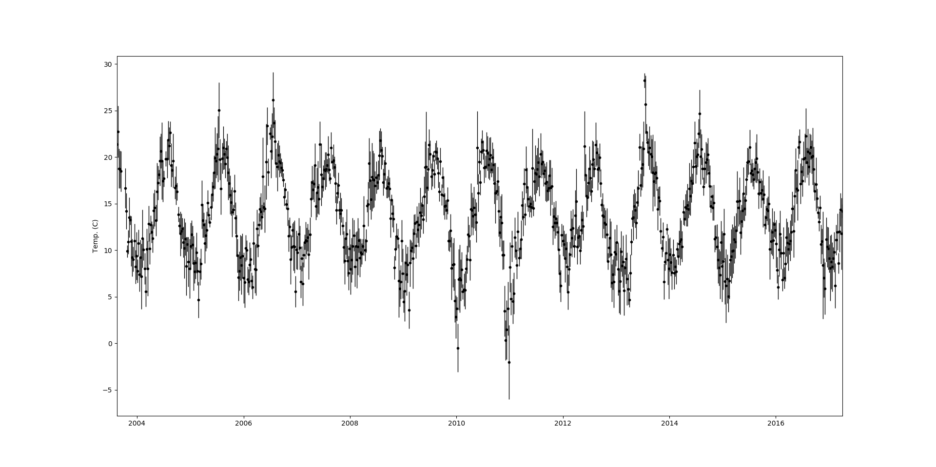
So our dataset is temperature, $y$, vs week number, $x$, with some uncertainty attached to each point, $u$. The most noticable feature of this data set is the periodicity, unsuprisingly it gets hot in the summer and cool in the winter. Since we’re dealing with data with a very clear periodicity we want to pick a kernel that will reflect this. The periodic kernel in George is,

This kernel will have a structure whereby points that are a distance of $1/P$ from one another will have a large covariance, like this

We can instantiate that kernel in George and evaluate the log-likelihood of our data under this model, as well as its gradient,

kernel = 10 * kernels.CosineKernel(1/50)

gp = george.GP(kernel, mean=np.mean(y))
gp.compute(x, yerr=u)
print(gp.lnlikelihood(y))
print(gp.grad_lnlikelihood(y))

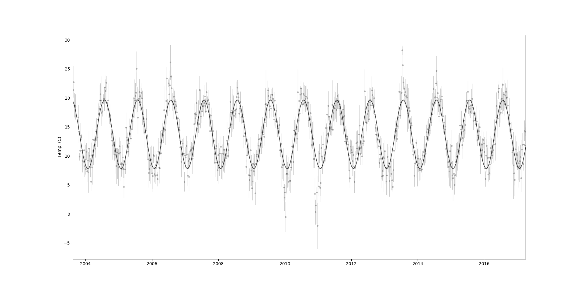
In reality it doesn’t really make sense to use just the periodic kernel, you’d probably want to take the product of this kernel with something else to allow for quasi-periodic oscillations. Using this kernel alone is equivalent to fitting a simple periodic model to the data, but that’s enough for the sake of this example.

Now that we’ve specified a model in George we can optimise the parameters of the kernel (the scaling factor and the period). As in our home-grown GP in the last post we’ll do this using the minimiser in scipy

def nll(p):
    gp.kernel.parameter_vector = p
    ll = gp.lnlikelihood(y, quiet=True)
    return -ll if np.isfinite(ll) else 1e25

def grad_nll(p):
    gp.kernel.parameter_vector = p
    return -gp.grad_lnlikelihood(y, quiet=True)

gp.compute(x, yerr=u)
p0 = gp.kernel.parameter_vector
results = opt.minimize(nll, p0, jac=grad_nll)

This shouldn’t have too much trouble getting to a solution, provided you’ve made a judicious choice for the initial parameters. In the end we get something like this,

One nice thing that we can do with George, as with GPFlow and PyMC3, is rather than direcly optimising for the maximum likelihood parameters we can sample from the likelihood and use an MCMC solver to accurately model the uncertainty in the hyperparameters.² To do this I’ll use emcee, a Hamiltonian Monte Carlo sampler by the same authors as George.³ Implementing the MCMC algorithm in emcee is pretty straightforward. We can build a log-likelihood which incorporates our priors

def lnprob(p):
    if (0 > p[1:]) | (p[1:] > 1):
        return -np.inf
    gp.set_parameter_vector(p)
    return gp.lnlikelihood(y, quiet=True)

In this case I’m using a uniform prior on the period. We then set-up the walkers (emcee uses ensemble of samplers which share information) in a small ball around our initial point and let them run.⁴

nwalkers, ndim = 6, len(gp)
sampler = emcee.EnsembleSampler(nwalkers, ndim, lnprob)

p0 = gp.get_parameter_vector() + 1e-4 * np.random.randn(nwalkers, ndim)

print("Running burn-in")
p0, _, _ = sampler.run_mcmc(p0, 100)

print("Running production chain")
sampler.run_mcmc(p0, 500)

We run burn-in first to let the chain ‘forget’ where it started from, then we run the production chain that we’ll treat as our posterior. All this takes a lot more computation than the straightforward optimisation we did before (though still not that much on this small problem), but in some sense it’s more honest. Rather than simply looking at the GP with the single best, parameters we can now look at the distribution of GPs with parameters consistent with our data. Also, we can get an estimate of the period of our data, $52.5$ weeks $\pm3$ days , which seems fairly reasonable to me.

GPs is a huge area, and growing all the time as they see more and more use in fields like astrophysics. They’re powerful, flexible, and are incredibly useful in situations where we want to accurately quantify uncertainty, or where we want to learn from small datasets. In these blog posts I’ve only covered the headlines, what they are, how they work, and why they’re useful, and hopefully I’ve done it in a way that was easy enough to follow. If you want to know more about the topic you can’t do a lot better than Rasmussen and Williams Gaussian Processes for Machine Learning book, which is brilliant and, conveniently, is free online.