Norms

What’s in a norm?

A norm is essentially a way of summarizing a set of numbers in a single value. From a geometric perspective if we consider our list of numbers to a be a vector in some space, then the norm is a way of attributing some sense of length to this vector. When dealing with measure theory and probability we often find ourselves working with vectors that live in Lebesgue spaces, and these spaces are equipped with a specific class of norm, called L$^p$-norms. These norms have a special form, given a vector $x$

This should look kind of familiar, it contains as a special case (L$^2$) the good old Euclidean norm that we all know and love

as well as defining an infinite family of other norms, one for every value of $p$. Looking at some of these norms we can quickly see their connection with statistics. Let’s say we have a list of numbers and we want to find a value, which we’ll call $s$, that well summarizes this list. We begin by subtracting the summary value from each value in the list, and we then apply a norm to the result, with this value being a measure of how good our summary is,

Starting with the L$^0$-norm, how would we choose $s$ such that $\Delta$ is minimized? The L$^0$-norm is just the count of the number of non-zero elements our list¹, so it should be clear that the $s$ that minimizes $\Delta$ is the value that appears most often in the list. In other words the value that best summarizes a list of numbers, if you use the L$^0$-norm as your metric, is the mode.

We can follow a similar line of reasoning with the L$^1$-norm. The L$^1$-norm measures the sum of the absolute values of the vector, in our case the sum of the distances between $x_i$ and $s$. Following on from the L$^0$-norm we see that the value for $s$ that minimizes the L$^1$-norm is the median of the list. Doing this once more for the L$^2$-norm, the $s$ that works best is the mean of the list. This is pretty cool, we can see that some of the basic statistics that we use arise directly from trying to minimize the distance between a single value and a list of values, as measure by different L$^p$-norms.²

It seems that there is a natural extension here, rather than trying to minimize the difference between a value and a list, we could look at minimizing the difference between two lists for the case of linear regression

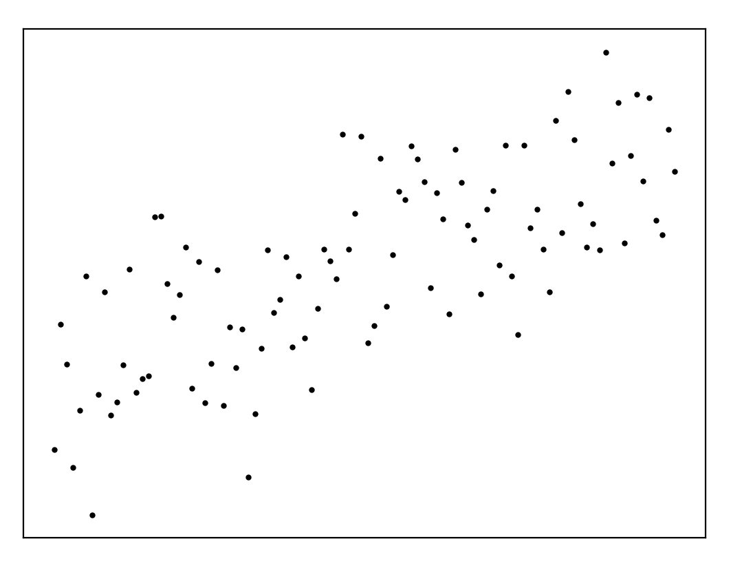
So we want to find some set of values, $m$ and $c$, that minimizes the difference between $x$ and $f(x)$ as measured with some norm. Let’s generate some linear data and work through some examples,

def get_data():
        x = np.linspace(-1, 1, 100)
        y = np.random.normal(x, 0.5)
        return x, y
plt.plot(*get_data(), '.k')

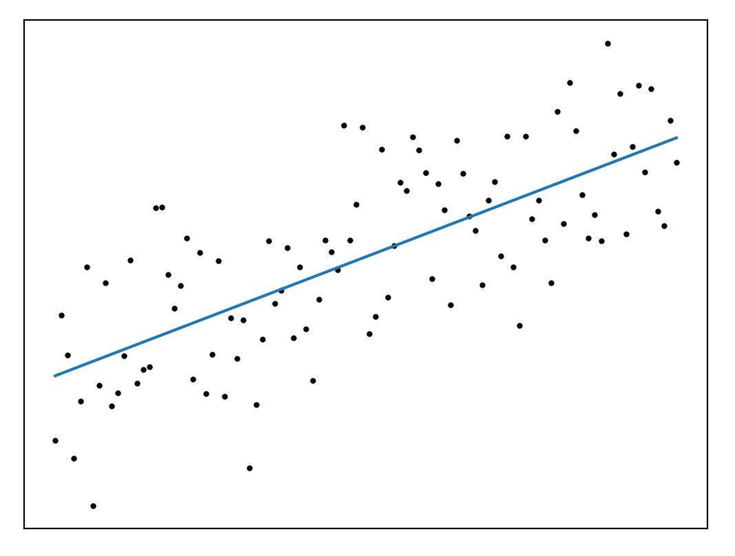
If we start with the L$^2$ norm,

we have the familiar squared error, and the problem we’re solving is Ordinary Least Squares (OLS). Thanks to Gauss we know that we can solve this problem analytically,

def ols(x, y):
        x_ = np.vander(x, 2)
        mp = np.linalg.inv(x_.T.dot(x_))
        w = mp.dot(x_.T).dot(y)
        return x_.dot(w)

Since this norm is convex and well-behaved we could also solve this by gradient descent, and get the same answer

def model(theta, x):
        m, c = theta
        return m * x + c

def l2(theta, x, y):
        return ((y - model(theta, x))**2).sum()

res = minimize(l2, [1, 1], args=(x, y))

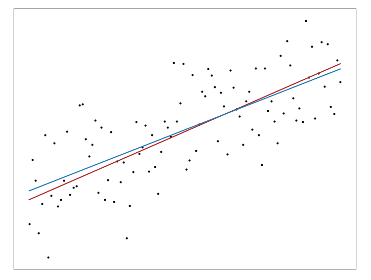
While the L$^2$-norm is by far the most well-known for regression the L$^1$-norm, often called Least Absolute Deviation, or Robust Regression, is also commonly used. The robustness of this method comes from the fact that it is less sensitive to outliers than the L$^2$-norm, which sums the squared difference between each prediction and observation and so weights large differences more heavily. Unfortunately there’s no analytical solution for L$^1$ regression, and even more unfortunately we can’t solve it by gradient descent since the L$^1$-norm isn’t differentiable everywhere.³ Thankfully we can turn to the dark arts of Linear Programming to solve this problem, and we can implement our solution using the Python bindings for the CVX package.⁴ We can plot up our new predictions (in red) and see that we get a slightly different estimate,

from cvxpy import Variable, Minimize, Problem, norm1

def lp(x, y):
        m, c = Variable(), Variable()

        obj = Minimize(norm1(y - (m * x + c)))
        prob = Problem(obj).solve()

        return m.value * x + c.value

Tying back to our observation about the connection between these norms and summary statistics, what we’re doing with these two types of regression is predicting a particular statistic conditional on the observations – which is to say OLS predicts the mean of $y$ conditional on $x$ and and L$^1$ regression predicts the median. Under this interpretation we can define a broader class of methods called quantile regression, where we attempt to predict the conditional $n^\rm{th}$ quantile of a distribution.

It seems sensible to continue our look at norms for regression, and go to L$^0$ regression.⁵ The problem with L$^0$-norm regression is that it reduces to an intractable combinatorial problem, you’re trying to find the line that goes through the most points. I’ve never heard of anyone using L$^0$ regression, but maybe there are some cool use cases out there I’ve missed.

To close off let’s go entirely in the other direction and look at L$^\infty$-norm regression. This norm is defined as the maximum of the vector we’re given,

In other words minimizing this norm means finding the line that has the smallest maximum distance to any other point. This problem isn’t intractable like the L$^0$ case, it actually has a couple of very simple expressions as linear programs.⁶ We can implement a solution using CVXPy as before

def lp(x, y):
        m, c = Variable(), Variable()

        obj = Minimize(normInf(y - (m * x + c)))
        prob = Problem(obj).solve()

        return m.value * x + c.value

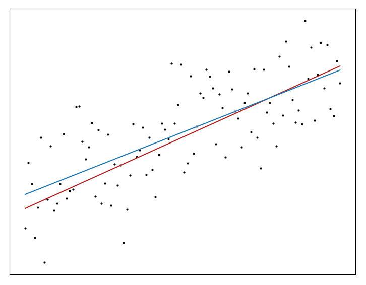
The line in red here is the line with the smallest maximum distance from any point.

We can extend our discussion further at this point by looking at using the norms to enforce regularization – for instance using an L$^2$ norm for regression but adding a penalty term which applies the L$^1$ norm to the model parameters. But that’s another blog post.