The difference between right and wrong

In classification problems there are a lot of metrics that you can look at, but they all have blind-spots. It can be really easy to build a model that scores well on some metric but ends up not being useful to the problem you’re trying to solve. When you see a metric for some model it’s useful to bear in mind what this metric measures, and equally importantly, what it doesn’t.

Confusion Matrix

Let’s say we’re dealing with a binary classification problem, we have some data, $X$, and some binary labels $Y \in (0,1)$. We’ve built a model that, given $X$, comes up with a classification $\hat{Y} \in (0,1)$. How do we measure the performance of that model on new data? Well there are 4 possible outcomes

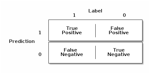
This is called a confusion matrix, and from it we can see there are 2 ways for us to be right, a true positive (label a $1$ as $1$), or a true negative (label a $0$ as $0$). Unfortunately there are also 2 ways for us to be wrong, a false positive (label a $0$ as $1$) a false negative (label a $1$ as $0$). These are often called type I and type II errors respectively.¹

These 4 values tell us everything we need to know about a given classifier, but how do we compare 2 classifiers to one another? For that it would be useful to have a single number, a metric; a better classifier gets a bigger number. But there’s the rub, the issue with all metrics boils down to the fact that you can’t compress all of the information in this $2\times2$ matrix into one number without losing something along the way. This is why we have a whole lot of metrics, each answers a different question, and why picking the right one for the problem you’re working on is so important.

Accuracy

Probably the most straightforward metric is accuracy, this is simply the fraction of examples that got the correct label,

If someone asked you to come up with a metic this is probably the first one you’d suggest, but unfortunately it’s easily fooled. Let’s say we have a useless model that just labels everything with $1$. If we test it with data that’s 50/50 split between $1$ and $0$ we’ll get accuracy 0.5. Bad model, bad score. Reality rarely gives us such nice data, what happens if we get data that’s biased 90/10? Well now our model gets 0.9 accuracy! It’s just as useless as it was before, it still has no predictive power, but now it has really high accuracy. Maybe we need more subtle metrics.

Precision & Recall

Two common metrics are precision and recall (also called sensitivity). These are defined as:

Precision and recall have nice probabilistic interpretations,

So precision is the probability that a something labelled a $1$ is really a $1$, and recall is the probability that a true $1$ will be labelled as such. Precision is a probability conditioned on your estimate of the class label, and so like accuracy it will vary if you use your classifier on different populations with different biases – since recall is conditioned on the class label probability it will remain the same as the population changes:

def dilute(y, p=0.9):
        '''
        Given a value and a dilution factor,
        this will give True for all 1's
        and False for a random p % of 0's
        '''
        if (y == 1) or (np.random.rand() > p):
                return True
        return False

mask = list(map(dilute, y))

y.mean()       # 0.5
y[mask].mean() # 0.909

precision(y, y_hat) # 0.871
recall(y, y_hat)    # 0.869

precision(y[mask], y_hat[mask]) # 0.985
recall(y[mask], y_hat[mask])    # 0.869

As you can see in the above example, using the same labels and classifications we can get very different precisions by evaluating on different sub-populations of the data. This isn’t necessarily a drawback however, the question being answered by the precision, “What is the probability that this is a real hit given my classifier says it is?”, is the relevant question in a lot of applications. If you’re working in a field where the positive class is what you really care about, and the “background” probability is well understood, then precision is extremely relevant – if you’re a doctor and a high-precision test tells you someone’s sick, for instance, that’s useful information.

But as ever it’s worth remembering what has been ruled in and what has been ruled out by a given score on a metric. By applying Bayes Rule to the definition of precision we can see that we could construct a high precision/low recall classifier if $P(\hat{Y} = 1)$ is small, i.e. if we have a high false negative rate. In the case of the doctor knowing our test has high precision gives us confidence in diagnosing someone who has gotten a positive result, but it doesn’t rule out a lot of people who got negative results being sick too. In order to quantify that we want a metric which relates to the opposite property, if you test negative then we can rule out you being sick with high confidence. This related property is called specificity $(P(\hat{Y} = 0 \vert Y = 0))$.

AUC

One of the most often reported metrics in machine learning is ROC-AUC. An ROC curve is computed by varying the threshold at which the classifier returns a positive label,² and plotting the true positive rate (TPR) against the false positive rate (FPR) for each of these classifiers. This will give a curve like this

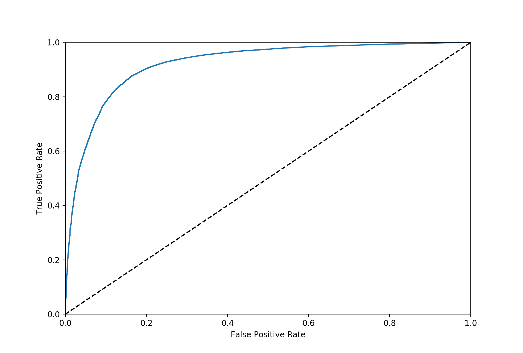
In the worst case scenario (a random classifier) the TPR will be equal to the FPR, you’ll get as many wrong as right, and the ROC curve will follow the dotted line. For a classifier that’s doing its job this curve will always be above the dotted line, its TPR will be greater than its FPR – if the FPR is greater than the TPR then your classifier has discriminative power but it’s applying the wrong labels.

Measuring the area under this curve we see that a random classifier will score $0.5$, a perfect classifier will score $1$. The ROC-AUC, sometimes called the concordance, also has a nice probabilistic interpretation, it is the probability that a randomly selected positive example will be given a higher score than a randomly selected negative example. The ROC-AUC has a couple of useful properties, for one it’s fairly insensitive to class imbalance. Another important point about ROC-AUC is that it measures the ability of a classifier to produce good relative scores, it doesn’t need to produce well-calibrated probability estimates to get a high ROC-AUC.

You’ll also often see a precision-recall curve, which is based on the same premise as an ROC curve, but with precision and recall on either axis. A good PR curve is the other way around to a ROC curve; a good ROC curve should go to the top left, a good PR curve to the top right

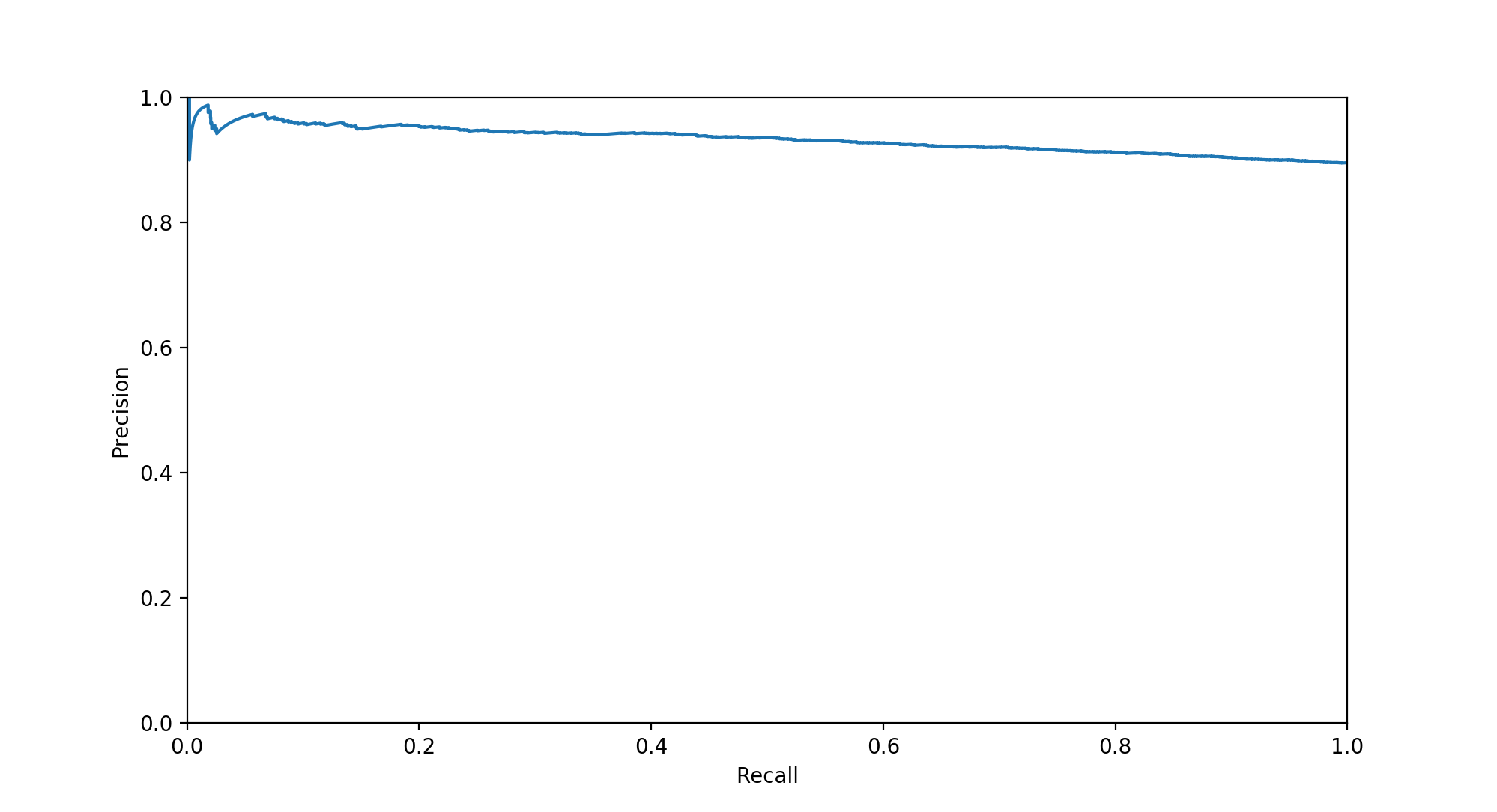
Unfortunately the area under the PR curve doesn’t have any nice interpretation that I’m aware of, but it’s a metric you’ll often see since it’s insensitive to the true negatives. Since the true negatives are ignored by PR-AUC (they enter the ROC through the FPR³) it will be more useful in situations where true negatives aren’t important. The relationship between the PR and ROC – along with some interesting observations about the parts of PR space that you can’t get to – is explored in this paper.

Conclusions

There are a lot of metrics out there and I’ve only covered the headlines here, this paper has a great summary of some of the zoo of metrics available to judge a classifier. The general message for all of these classifiers is caveat emptor; be aware of the question you’re trying to answer and pick a metric that addresses it.

If what you’re interested in doing is building a classifier that will perform equally well in both the positive and negative cases then ROC-AUC is probably the most relevant metric, as well as the most interpretable because it can be directly related to cost/benefit analysis. However if you’re not so bothered about the negative class and care more that every positive prediction has high probability of being correct, and that you have a high probability of returning every positive case out there, then PR-AUC is the way to go.