Can you judge an album by its cover?

They say not to judge a book by its cover, but what about an album? What does the cover tell you about the contents, can you reliably figure out the genre of an album just by looking at it? My feeling is that you could, to some extent. If you showed me an album cover, out of context, I feel like I could take a decent stab at the kind of music that’s on it. So I wrote some code to try to quantify this.

Everything below can be found in this repo.

Data

The first thing we need is some data. Thankfully you can find almost anything you want on the internet, and for this task I came across this data set. This file has links to 10,000 album covers from 10 genres (1,000 each), collected using the Bandcamp API. It’s just a matter of walking through that file and pulling down the images. Easy.

Now that we’ve got the data, the best place to start is by taking a look at it, a quick sight-check to make sure that we’ve got what we expect. Andrej Karpathy wrote a good blog post where he tried to hand classify some of the images, it’s well worth a read. Eye-balling the data like this is a really useful way to get a qualitative impression of things, and to get an idea of where a classifier might succeed or fail. To do that I wrote a little script to pull out and plot up some random images

def pick_images():

        dirs = glob.glob('data/train/*')
        imgs = []
        for d in dirs:
                fs = glob.glob(f'{d}/*')
                f = np.random.choice(fs)
                imgs.append(f)

        return sorted(imgs)

def plot_images():

        imgs = pick_images()

        fig = plt.figure()
        columns = 5
        rows = 2
        for i in range(1, columns*rows +1):
                path = imgs[i -1]
                genre = path.split('/')[2]

                img = Image.open(path)

                fig.add_subplot(rows, columns, i)
                plt.imshow(img)
                plt.title(genre)
                plt.axis('off')

        plt.show()

Running this gives something like:

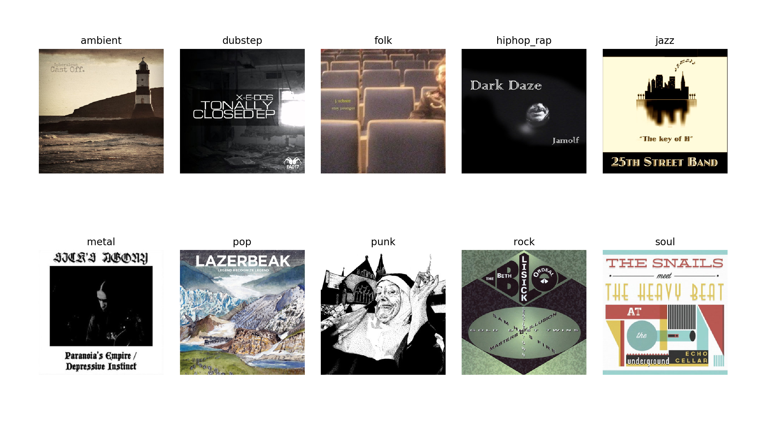
How many of those do you reckon you could match to the right label? Not so easy is it? Looking at a few plots like this you can start to build up an intuition for the job at hand. It looks like metal and dubstep might be easy enough to segregate from the others, and you could probably pick out hip-hop too - rock, folk, and soul all look really alike. You could argue that maybe these labels aren’t ideal for the task at hand, maybe we could make things easier by merging jazz and soul, or metal and punk - these strike me as genres with some overlap between them, though I’m sure their fans would disagree. It feels a bit like cheating to cut corners though, so I decided to stick with the labels we have.

Colour Classifiers

Based on taking a look at the data I feel like one of the most useful features might be the colour of the image - punk and metal are mostly black and white, pop is a bit more colourful - so let’s begin there. The best way I could think to use the colour was to make a histogram of the image in HSV (Hue, Saturation, Value) colour space. OpenCV gives us a handy tool for doing this,

def extract_color_histogram(image, bins=(8, 8, 8)):
        '''
        extract a 3D color histogram from the HSV color space using
        the supplied number of `bins` per channel
        '''
        hsv = cv2.cvtColor(cv2.imread(image), cv2.COLOR_BGR2HSV)
        hist = cv2.calcHist([hsv], [0, 1, 2], None, bins,
                [0, 180, 0, 256, 0, 256])

        cv2.normalize(hist, hist)
        return hist.flatten()

This function takes in an image, a ($350^2 \times 3=$) 367500 element array, and spits out a ($8^3=$) 512-dimensional feature vector. Now that we have every image as a point in 512d space we can start classifying.

It’s always a good idea to start off with the simplest classifier to get a baseline performance. The simplest possible classifier here is just to find an image’s nearest neighbours in this colour space, and give it the same label as those. To do this I used Annoy, which searches for points in the space that are closest to a query point. In high dimensions this is an expensive operation, so Annoy solves the problem approximately, trading a little accuracy for a big speed-up. My classifier takes in the training set and records their locations in colour space. Then when you ask for the genre of a query image it takes the 10 closest points in the training set and gives the query image the most common label among those, i.e.

prediction = Counter(train_labels[i] for i in 
                       annoy.get_nns_by_vector(query, 10)).most_common()[0][0]

Unfortunately this doesn’t perform too well, it only classifies around 13% of images correctly. If you just guessed randomly you’d get 10%, so this isn’t great. But it gives us starting point to improve from.

A easy improvement is just to stick on a better classifier and see if we do better. Taking out the nearest neighbours and replacing it with an out-of-the-box XGBoost classifier we see some improvement, but not a lot. It now gets up to ~17% accuracy. I’m sure with some hyper-parameter searching and some more attention to the colour features would give us some incremental gains, but maybe the colour histograms aren’t the best approach. Let’s see what happens if we use all of the pixel level image data.

CNN

Rather than trying to make features from the image, a better approach might be to hand the image to a convolutional neural net and let it do the job for us. The CNN takes the entire image as input and passes it through a series of convolutional filters, at each layer building more abstract features. The whole net is differentiable so it can be trained by backprop to pick out and combine the most relevant features, to make the best higher order features, and finally to make a classification. That was very handwavy but I guess you’re probably fairly familiar with CNNs, if not CS231 is a good place to start.

Training a CNN is a pretty expensive operation, and would be totally infeasible on a data set of this size, we’d overfit horribly. Thankfully we don’t have to go through the trouble, we can just use the weights of a pre-trained network like VGG16, a process called transfer learning. The VGG16 network won the 2014 ImageNet Challenge, and the weights are published online. In general networks like these have two parts, a series of convolutional layers that produce the high-level features, followed by a couple of fully-connected layers that take the convolutional features and make a prediction. We can chop off the top part of the network, keeping of the convolutional base and retraining the fully-connected layers for our prediction task. The outputs of the convolutional base won’t be optimised for our specific task, but the hope is that the features that were useful in the ImageNet Challenge will also be useful in making album predictions.

In this case I replaced the fully-connected component of the net with a super simple one-layer network; 256 hidden units, a little dropout, trained with cross-entropy:

def net(inshape, outshape):

        model = models.Sequential()
        model.add(layers.Dense(256, activation='relu', input_dim=inshape)
        model.add(layers.Dropout(0.5))
        model.add(layers.Dense(outshape, activation='softmax'))

        model.compile(optimizer=optimizers.RMSprop(lr=1e-4),
                loss='categorical_crossentropy',
                metrics=['categorical_accuracy'])

        return model

Using this net doubles our prediction accuracy, we’re now at ~33%! You can see the prediction accuracy by genre pair in the confusion matrix

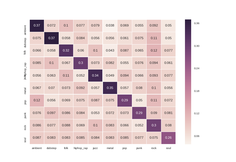
Looking at this confusion matrix we see some interesting patterns. It looks like soul albums are pretty hard to classify, we only get about 1 in 4 of these right. On the other end of the spectrum, we’re able to get almost 40% of ambient albums right, which isn’t bad at all. We almost never mistake dubstep for soul, ambient for punk, or jazz for metal, which is all both really encouraging and in line with what you’d guess by looking at the data. Given how tough a classification problem this is, I’d say this net is doing a pretty good job.

Conclusions

So to go back to our original question, it seems you can correctly judge an album by its cover about a third of the time. I guessed to begin with that the colour of the cover would be well correlated with genre, and you can make a reasonably good classifier based on that idea. The old-fashioned approach to improving this classifier would have been by engineering more complex features, incrementally increasing the accuracy that way. But we don’t have to limit ourselves to hand-crafted features, we can throw all of the data into a CNN and see what we get out. Unfortunately training an end-to-end neural network would be infeasible for such a small data set - you can’t learn 140,000,000 parameters from 10k examples.¹ Thankfully we don’t have to learn all of them, transfer learning to the rescue! Taking a ready-trained CNN and tweaking some of the parameters to tailor it to our task we can get really great performance at very little cost. I wasn’t sure that this approach would work, I thought that the intra-genre variability of image contents/structures would be swamped by inter-genre variability, but I underestimated how good CNN’s are at picking out these features. We could probably improve the performance of this classifier by deepening the fully-connected network, and working a little harder on hyper-parameter searching, but we have to stop somewhere and to be honest I’m pretty happy with how well this net works on what is a non-trivial problem.