Optimal Binning
Making a histogram out of some data is one of those things that sounds really straightforward at first and gets progressively more complicated the more you think about it. Defining things clearly, lets say we have a vector, $x$, of $n$ observations, and we want to break up the number line into a series of buckets and count up how many $x$’s fall in each one. How would we do that?
The first thing you’d probably do is create $k$-evenly spaced bins but this brings up an immediate
issue, what value should we choose for $k$? It’s clear that the best $k$ (whatever that means) will
be different for different data sets, so what do we go with? There are a couple of heuristics to the
rescue here, and if you call np.histogram you’ll end up employing one of the following. The
simplest is Sturges’ formula, which sets $k$ to
be:
Since this is solely a function of the number of data points it’s not very useful in the case that $n$ is small, it’ll bin really coarsely. A slightly more complicated, and slightly cleverer choice is given by the Freedman-Diaconis Rule:
\[h = 2 \frac{\rm{IQR}(x)}{n^{1/3}}\]where $h$ is the width of the bins, and IQR is the interquartile range of x, i.e. the distance
between the 25th and the 75th percentiles, the range into which the middle half of the data fall.
This seems like a sensible quantity to have in an equation like this, and it turns out to be quite
useful, even giving us some guarantees about the sensitivity of this binning to outliers. As I
said, if you’re using np.histogram you’re getting one or the other of these, whichever
gives more bins. Most people would be happy enough with that but it does seem like we’re leaving
the table a little early here, surely we can do better than these fairly simple approaches. For
instance maybe we can vary not just the number of bins but also their sizes.
It turns out that making optimal bins is something that’s useful to people in a lot of different fields. For instance people in the business of making credit scorecards were/are pretty interested in this in order to help in making more accurate predictive models while maintaining interpretability. Astrophysicists (full disclosure, I fall into this bin) are interested in the best way to group together photon counts so that they get the best trade-off possible between signal and noise. People looking at time-series might be trying to group data together in a motivated way to look for change points. So as it happens there’s quite a bit of literature on the topic.
From the astrophysical domain there are two particularly interesting papers that I’ve come across, one by the Scargle, of periodogram fame, and one by Hogg. Scargle’s paper is really fascinating, coming at the problem from a Bayesian perspective, and uses a dynamic programming algorithm to build up an optimal set of bins for a given data set. The paper itself is really clear, and even comes with a Matlab implementation of the algorithm. Jake Vanderplas has an accessible write-up on his blog. One of the downsides of Scargle’s algorithm is the complexity, scaling as $\mathcal{O}(N^2)$ in the number of data points. This isn’t bad given that it’s choosing the optimal configuration of bins out of $2^N$ possibilities, but for a reasonably-sized data set a quadratic scaling is a bit of a killer. As a result I decided to make use of Hogg’s model, and put an algorithm together based on that.
It’s always a good idea to have a well-defined model as a starting point in order to motivate the questions we’re asking. A good model for a histogram comes from the observation that in the limit of infinite data the histogram converges to the PDF. So the best histogram of a set of data is the one that matches the PDF as well as possible given how much data we’ve seen. A different way of phrasing this is that the best histogram will best predict where future data will land. As such we might start with a model like this: given a new observation we would expect it to fall into bin $i$ with probability given by the proportion of the observations we’ve already seen go into that bin. Mathematically:
\[p(i) = \frac{N_i}{\sum N_i}\]where $N_i$ is the number of observations in bucket $i$. This is not a great model though, because it a priori assigns 0 probability to the regions where we haven’t observed any data yet (by chance), and if (by chance) an observation falls into that region the model will break. A better model would include a small smoothing parameter1, $\alpha$, to make sure that we put some mass on regions where we’ve not seen anything yet
\[p(i) = \frac{N_i + \alpha}{\sum N_i + \alpha}\]This is a better model, and using it we can produce a Leave-One-Out cross-validation log-likelihood:
\[L = \sum_j w_j \ln \left(\frac{W_i + \alpha - w_j}{h_i(\sum_k W_k + \alpha) -w_j} \right)\]Where $j$ designates a sum over points, $w_j$ is the weight associated with point $x$, $W_i$ is the sum of all the $w$’s in bin $i$, and $h$ is the width of bin $i$. This is the general form, but in the case that our data have binary weights (the case where $w_j = 1 \; \forall j$ is a histogram) we can greatly simplify this equation to a (much more efficient) sum over bins
\[L = \sum_i W_i \ln \left(\frac{W_i + \alpha - 1}{h_i(\sum_k W_k + \alpha) - 1} \right)\]Great, so now we have a way of scoring a given histogram, how can we use it to find the optimal binning? To do this I implemented a simple greedy algorithm that’ll be familiar to people used to binning by GINI or entropy, a bit like the algorithm used in growing decision trees. It goes like this:
1) Split the domain of $x$ into $n$ even bins
2) Compute $L$
3) For each of the $n-1$ bin-edges, remove the edge whose removal most increases $L$
4) Repeat until $L$ will be decreased by merging any more bins
By this process we begin with a fine binning of $x$ and we keep merging bins until each pair of adjacent bins are in some sense optimally different from one another. The nice thing about this simple model is that it can be implemented really easily (no dynamic programming required) and it has complexity $\mathcal{O}(N_{bins}^2\log(N_{data}))$. Great!
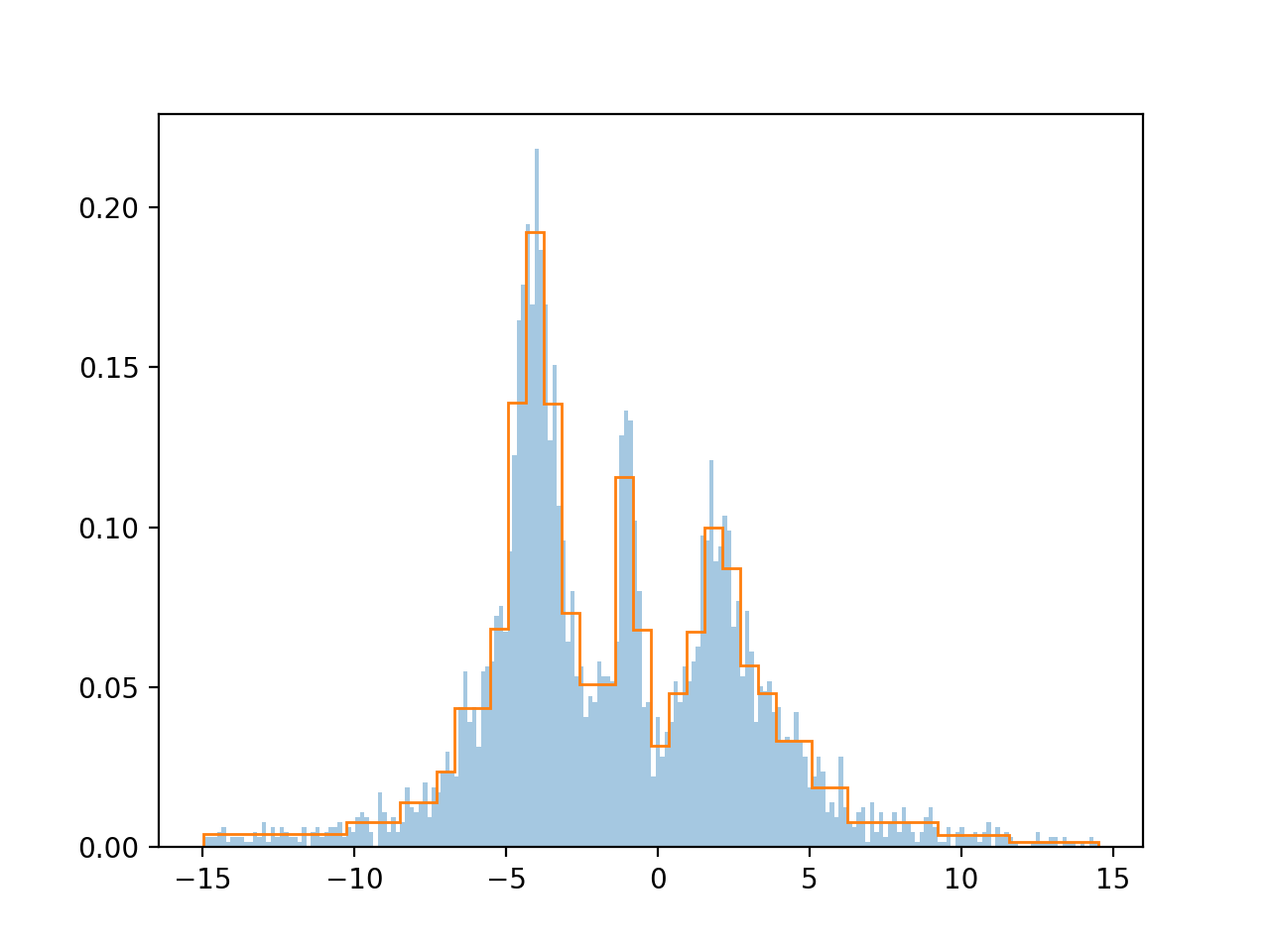
All isn’t rosy in the garden however, there are drawbacks to this method. Since we start off with $n$ even bins and we only ever remove bin-edges, never adding or moving any, we end up with edges on integer fractions of the range of $x$, which may not be optimal. Secondly, since the algorithm is greedy it will drive directly into the first local minimum it sees, and it will never pass through a low-likelihood region to get to a higher likelihood one, e.g. if we have 3 bins where 1 would be optimal, but merging any pair would be worse than keeping the 3, then we’ll never get to the 1 bin optimal solution. These drawbacks are a shame, but on the whole it seems the histograms we arrive at are pretty good. The example below is what we get when binning some arbitrary Cauchy functions I’ve stuck together.
I’ve coded this up in a sklearn transformer here.
-
It occurs to me as I write this that this model is a lot like Good-Turing Smoothing. ↩